Sheet Arduino n.5 (V/I characteristic curve of a led)
[Lezione del 19 nov 2019]
Aggiornamento del 14 gen 2020
Un enorme ringraziamento al prof. Morresi che ha controllato il mio esercizio e scovato un errore nello sketch per Arduino: ho scambiato la V1 con la V2 alla linea 42.
Lo sketch corretto è il seguente:
1 2 3 4 5 6 7 8 9 10 11 12 13 14 15 16 17 18 19 20 21 22 23 24 25 26 27 28 29 30 31 32 33 34 35 36 37 38 39 40 41 42 43 44 45 46 47 48 49 | /* Embedded Systems Architecture - hardware
* application on 25th nov 2019
*
* measure ...
*/
#define TO_V (5.0 / 1024.0) // convert an analog UNO unit to V
#define TO_mV (5.0 / 1.024) // convert an analog UNO unit to V
#define RAMP_PIN 5
#define V1_PIN A0
#define V2_PIN A2
#define BUF_SZ 256
#define N_STEPS 256
#define TIME_BM 100
#define RD 100
#define FOREVER 1
unsigned int i;
int V1[BUF_SZ]; // mem V1 read from V1_PIN
int V2[BUF_SZ]; // mem V2 read from V2_PIN
void setup() {
pinMode(RAMP_PIN, OUTPUT); // this is our power to breadboard
Serial.begin(9600); // init the serial at 9600 baud
}
void loop() {
delay(1000);
Serial.print("MEASURE START time btwn measures: ");
Serial.println(TIME_BM);
for(i=0; i<N_STEPS; i++){
analogWrite(RAMP_PIN, i);
V1[i] = analogRead(V1_PIN);
V2[i] = analogRead(V2_PIN);
delay(TIME_BM);
}
Serial.println("MEASURE STOP");
delay(1000);
Serial.println("MEASURE PRINT START");
delay(1000);
for(i=0; i<BUF_SZ; i++){
Serial.print(V2[i] * TO_V, 4);
Serial.print(", ");
Serial.println( ((V1[i] - V2[i]) * TO_mV)/RD , 4);
}
Serial.println("MEASURE PRINT STOP");
analogWrite(RAMP_PIN, 0);
while(FOREVER){};
}
|
In queste condizioni il grafico per il led rosso è il seguente:
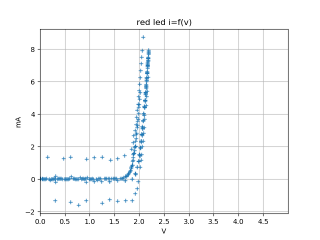
Come si vede, questo è decisamente più aderente al grafico ideale V-I di un led.
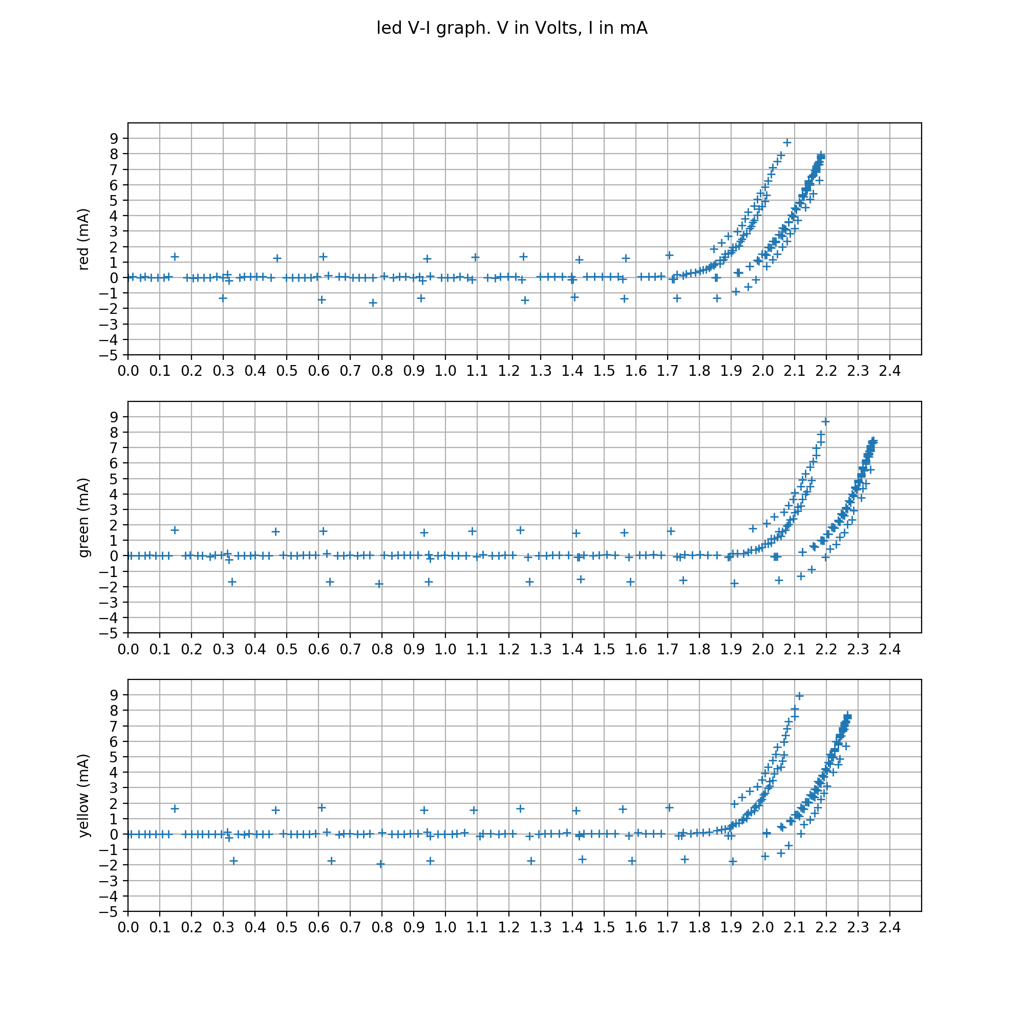
Se si vuole confrontare le curve per i tre led si ottiene il seguente:
V/I characteristic curve of a led
Vediamo la scheda della esercitazione n.5, che per lo scrivente è stato uno scoglio, non completamente superato. Il seguente video spiega perché:
Il dettaglio dello sketch è:
1 2 3 4 5 6 7 8 9 10 11 12 13 14 15 16 17 18 19 20 21 22 23 24 25 26 27 28 29 30 31 32 33 34 35 36 37 38 39 40 41 42 43 44 45 46 47 48 49 | /* Embedded Systems Architecture - hardware
* application on 25th nov 2019
*
* measure i=f(v) for a led
*/
#define TO_V (5.0 / 1024.0) // convert an analog UNO unit to V
#define TO_mV (5.0 / 1.024) // convert an analog UNO unit to V
#define RAMP_PIN 5
#define V1_PIN A0
#define V2_PIN A2
#define BUF_SZ 256
#define N_STEPS 256
#define TIME_BM 100
#define RD 100
#define FOREVER 1
unsigned int i;
int V1[BUF_SZ]; // mem V1 read from V1_PIN
int V2[BUF_SZ]; // mem V2 read from V2_PIN
void setup() {
pinMode(RAMP_PIN, OUTPUT); // this is our power to breadboard
Serial.begin(9600); // init the serial at 9600 baud
}
void loop() {
delay(1000);
Serial.print("MEASURE START; time btwn measures: ");
Serial.println(TIME_BM);
for(i=0; i<N_STEPS; i++){
analogWrite(RAMP_PIN, i);
V1[i] = analogRead(V1_PIN);
V2[i] = analogRead(V2_PIN);
delay(TIME_BM);
}
Serial.println("MEASURE STOP");
delay(1000);
Serial.println("MEASURE PRINT START");
delay(1000);
for(i=0; i<BUF_SZ; i++){
Serial.print(V1[i] * TO_V, 4);
Serial.print(", ");
Serial.println( ((V1[i] - V2[i]) * TO_mV)/RD , 4);
}
Serial.println("MEASURE PRINT STOP");
analogWrite(RAMP_PIN, 0);
while(FOREVER){};
}
|
Come detto nel video, il nucleo fondamentale è il ciclo da ln 31 a ln 36 in cui si effettua l’alimentazione con la tensione voluta (valori crescenti da 0 a 255), per poi effettuare le misure di V1 e V2, caricandole ciascuna in un prorpio vettore di 256 posizioni.
All’uscita del ciclo si manda sul monitor seriale il risultato delle misuraziono: la tensione di alimentazione V1 e la corrente del led, calcolata dividendo la tensione v1-v2 per la resistenza RD.
Possiamo copiare i dati stampati sul monitor seriale in un file txt creando praticamente un file CSV che contiene una misura V-I per ogni riga. Salvo le prime tre e l’ultima riga.
Un file del genere si plotta facilmente, ad esempio con il seguente programma Python:
1 2 3 4 5 6 7 8 9 10 11 12 13 14 15 16 17 18 19 20 21 22 23 24 25 26 27 28 29 30 31 32 33 34 35 36 37 38 39 40 41 42 43 44 45 46 47 48 49 50 51 52 |
help = '''python plot.py datafile led
where datafile is: v1, i
'''

import statistics as stats
import csv
import numpy as np
import os
from matplotlib import pyplot as plt
import sys

FN = 'n5-1.txt'
PLOT = 'i=f(v)'
LED = 'red led'

SNDX = 0
def sort_element(row):
    return row[SNDX]

def main(filename, plot):
    #read V1, I values from csv file
    with open(filename, 'r') as f:
        v = list(csv.reader(f, delimiter=','))  # V1, I

    v = v[3:-1]                                # no header(s) and tail
    v = [[float(e) for e in row] for row in v] # convert elements from string to float
    v.sort(key=sort_element)                   # and sort elements by v1 values

    #sys.exit(0)
    x = [v[r][0] for r in range(len(v))]       # v1 as x axis
    y = [v[r][1] for r in range(len(v))]       # I as y axis
    plt.plot(x, y, '+')                        # plot v1-I
    plt.title(LED + ' ' + plot)                # set plot title
    plt.xlabel('V')                            # set x axis limits
    plt.xlim([0,5])                            # set x axis limits
    #plt.ylim([-8,15])                         #- here we go in automatic mode
    plt.xticks(np.arange(0, 5, 0.5))
    plt.ylabel('mA')                            # set x axis limits
    plt.grid(True)
    #plt.show()                                # show interactively
    plt.savefig(os.path.splitext(filename)[0]+'.png', format='png') # show to file


if __name__=='__main__':
    #print(len(sys.argv))
    if len(sys.argv) > 1:
        FN =  sys.argv[1][:]
    if len(sys.argv) > 2:
        LED = sys.argv[2][:]
    main(FN, PLOT)
|
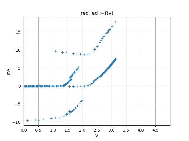
ottenendo grafici come il seguente (che illustra le misure per il led rosso):
Se si desidera confrontare le misure ottenute per i tre led: rosso, giallo e verde, possiamo usare:
1 2 3 4 5 6 7 8 9 10 11 12 13 14 15 16 17 18 19 20 21 22 23 24 25 26 27 28 29 30 31 32 33 34 35 36 37 38 39 40 41 42 43 44 45 46 47 48 49 50 51 52 53 54 55 56 57 |
help = '''python plot.py datafile led
where datafile is: v1, i
'''

import statistics as stats
import csv
import numpy as np
import os
from matplotlib import pyplot as plt
import sys

FN = ('n5-red.txt', 'n5-green.txt','n5-yellow.txt',)
PLOT = 'i=f(v)'
LED = ('red', 'green', 'yellow',)

SNDX = 0
def sort_element(row):
    return row[SNDX]

def main(filename, plot):
    #read V1, I values from csv file
    fig = plt.figure(figsize=[10,10], dpi=200)
    fig.suptitle('led V-I graph. V in Volts, I in mA') # global title
    ndx = 0
    axes = []
    for filename, color in zip(FN, LED):
        with open(filename, 'r') as f:
            v = list(csv.reader(f, delimiter=','))  # V1, I

        v = v[3:-1]                                # no header(s) and tail
        v = [[float(e) for e in row] for row in v] # convert elements from string to float
        v.sort(key=sort_element)                   # and sort elements by v1 values

        #sys.exit(0)
        x = [v[r][0] for r in range(len(v))]       # v1 as x axis
        y = [v[r][1] for r in range(len(v))]       # I as y axis
        if ndx == 0:
            axes.append(fig.add_subplot(3,1,ndx+1))
            axes[ndx].set_xlim(left=0, right=3.5)            # set x axis limits
            axes[ndx].set_xticks(np.arange(0, 3.5, 0.25))
        else:
            axes.append(fig.add_subplot(3,1,ndx+1, sharex=axes[0]))
        axes[ndx].plot(x, y, '+')                        # plot v1-I
        axes[ndx].set_ylim(bottom=-15, top=20)            # set x axis limits
        axes[ndx].set_yticks(np.arange(-15, 20, 5))
        axes[ndx].set_ylabel(color+' (mA)')
        axes[ndx].grid(True)
        ndx += 1

    #plt.show()                                # show interactively
    fig.savefig('graph.png', format='png') # show to file


if __name__=='__main__':
    main(FN, PLOT)
|
ottenendo:

Francamente ho passato molto tempo per cercare di spiegarmi il motivo per cui ottengo 4 curve, e non una. E non vi sono riuscito.
Prima di tutto ho dei valori proibiti, nel senso di correnti negative.
Inoltre sembra di avere a che fare con due curve, traslate verticalmente di circa -10mA. Con una interruzione nel mezzo della rampa in salita. Interruzione evidenziata da una coda di valori a corrente costante: una a 0mA e l’altra a circa 9mA.
Inizialmente ho pensato ad una costante RC implementata male. Ma mi sono dovuto ricredere: la resistenza è di 220Ohm (misurata) e la capacità di (dati dell’involucro) 470microF, pari a circa 0.1s. Valore più che ragionevole per tagliare le alte frequenze di un’onda quadra a 776.6Hz (misurata). Infatti la tensione a valle del condensatore è praticamente stabile, crescendo con regolarità al crescere del valore di PWM.
Purtroppo non ho un oscilloscopio per osservare il reale andamento nel tempo dei segnali. Cosa che mi permetterebbe di escludere un guasto hw dell’arduino.
In futuro, dovendo fare esercizi di collegamento tra due arduino, mi riservo la possibilità di provare con un secondo microcontrollore, per vedere se ottengo gli stessi andamenti.
Per ora voltiamo pagina!